Hybrid Search

Introduction

For a long time, search inside podcast apps felt broken to me. I rarely found what I wanted without fighting the search box. Then one day I wondered: what if search cared more about meaning and intent than the exact words I typed? What would the results look like? What would the experience feel like? Let's dig in and see what happened.

Context

To understand how search can become semantic, we need to understand vectors and embeddings.

Vectors and Embeddings

The gist is that vectors are a mathematical representation of words. In simpler terms, we turn a word into numbers a machine can understand. That numeric representation is what we call an embedding. This idea has been around in AI for a long time. It started with simpler methods, like counting words and other basic approaches, but those methods had many problems: meaning was hard to represent, different wording caused trouble, and so on.

Eventually, the common approach became training an AI model whose job is only to produce the best representation it can. Usually, "best representation" means placing things that are close in meaning near each other. In other words, the model starts to capture semantic and contextual relationships, then represent language in a useful way.

Note: embeddings are not limited to language. They are used in many places, including images.

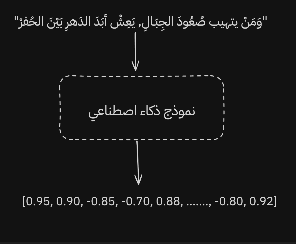The goal is to give the model a sentence and get back the best numeric representation it can produce.

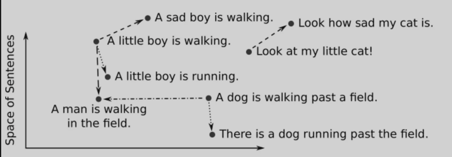
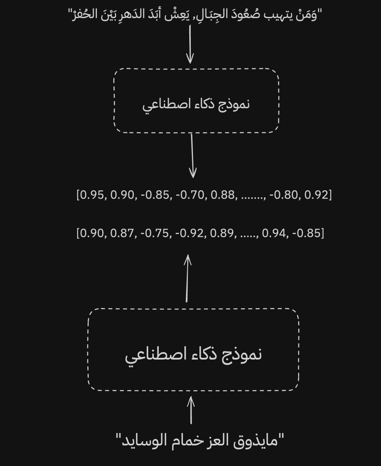When two sentences have close meanings, the model gives them close representations, even if one is formal Arabic and the other is colloquial.

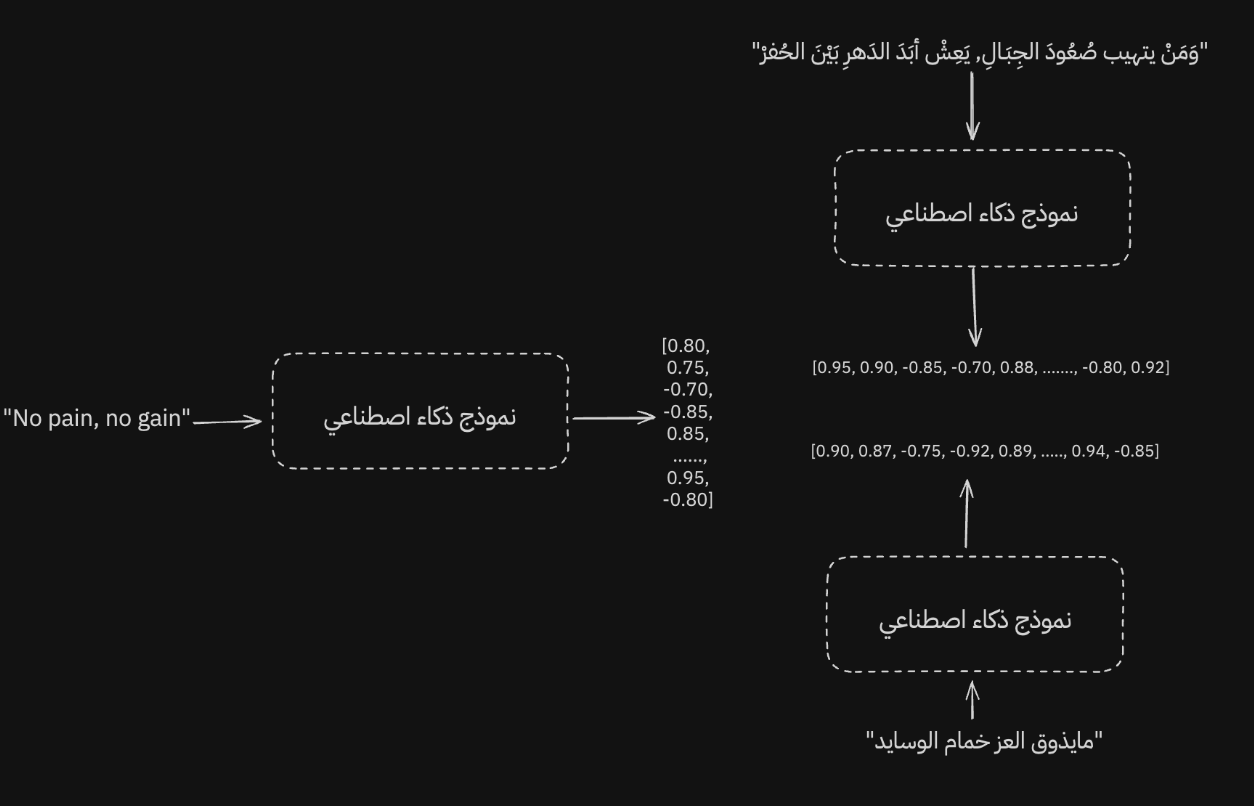A good multilingual model can keep representations close even when the language changes.

Not only that: the model can still produce similar representations even when we switch languages.

Of course, for a model to work well across multiple languages, this has to be part of training. The data and vocabulary need to be broad enough. So it is important to remember that not every model is trained for this goal. Some models are specialized for English, and their performance drops in other languages because they were not trained with multilingual representation in mind.

Now let's talk about some of the advantages that come from embeddings inside the embedding space.

Embedding Space

We have been talking about representing meaning. But what does that actually look like, and how can we interpret the model's output? Let's look at an example.

When we take the embeddings from the model and plot them on an x-axis and y-axis, they show up like this. Important note: this is a simplification. Embeddings usually have many dimensions, far more than we can comfortably visualize. So I reduced the output to two dimensions, x and y, to make it easier to understand.

Small note: in [-24, 420, 2.4, ...], every number inside the embedding is a dimension. Every extra number adds another dimension.

Now let's analyze the output. The sentences we chose are grouped near each other. We can measure that closeness in several mathematical ways. The most famous is cosine similarity, which measures the angle between two vectors. The smaller the angle, the more similar the vectors are. For example, if the angle is 12 degrees, cos(12º) is 97.8%. If the angle is perpendicular, 90 degrees, similarity is 0%, and so on.

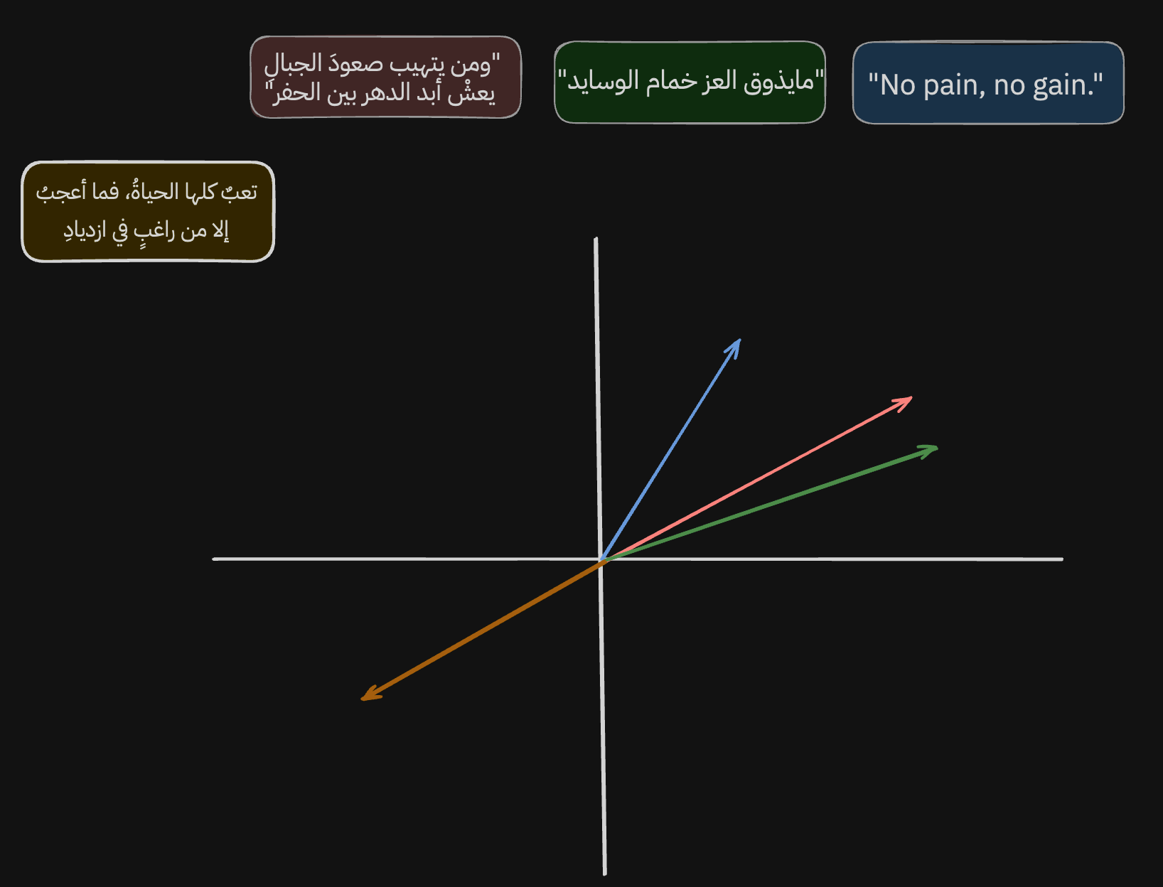
The interesting part is not only that embeddings let us measure semantic similarity between sentences. The model also learns to represent different meanings as different directions. Let me clarify what I mean.

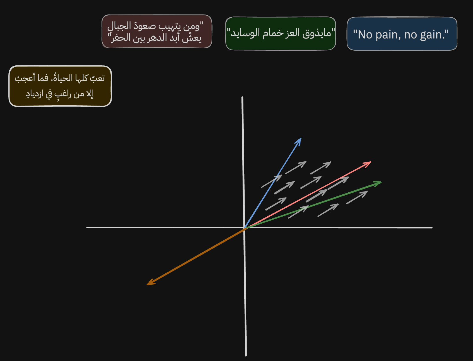
If we look at the gray arrows, we can see that the model learned to place sentences about hard work, effort, glory, and greatness in this area and direction.

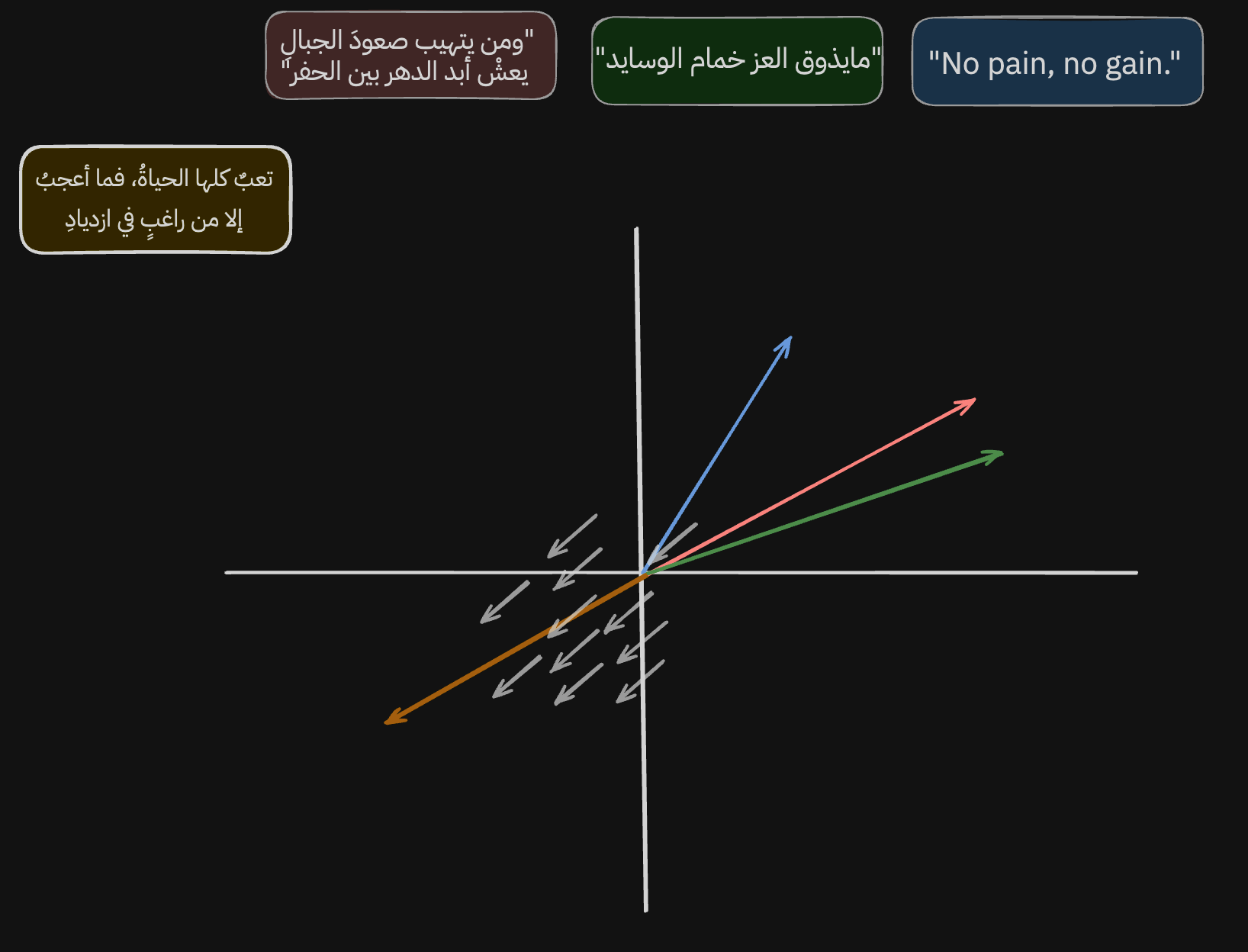
And if we look at the new line of poetry, we can see that the model learned the opposite direction too: sentences about defeat, brokenness, and laziness.

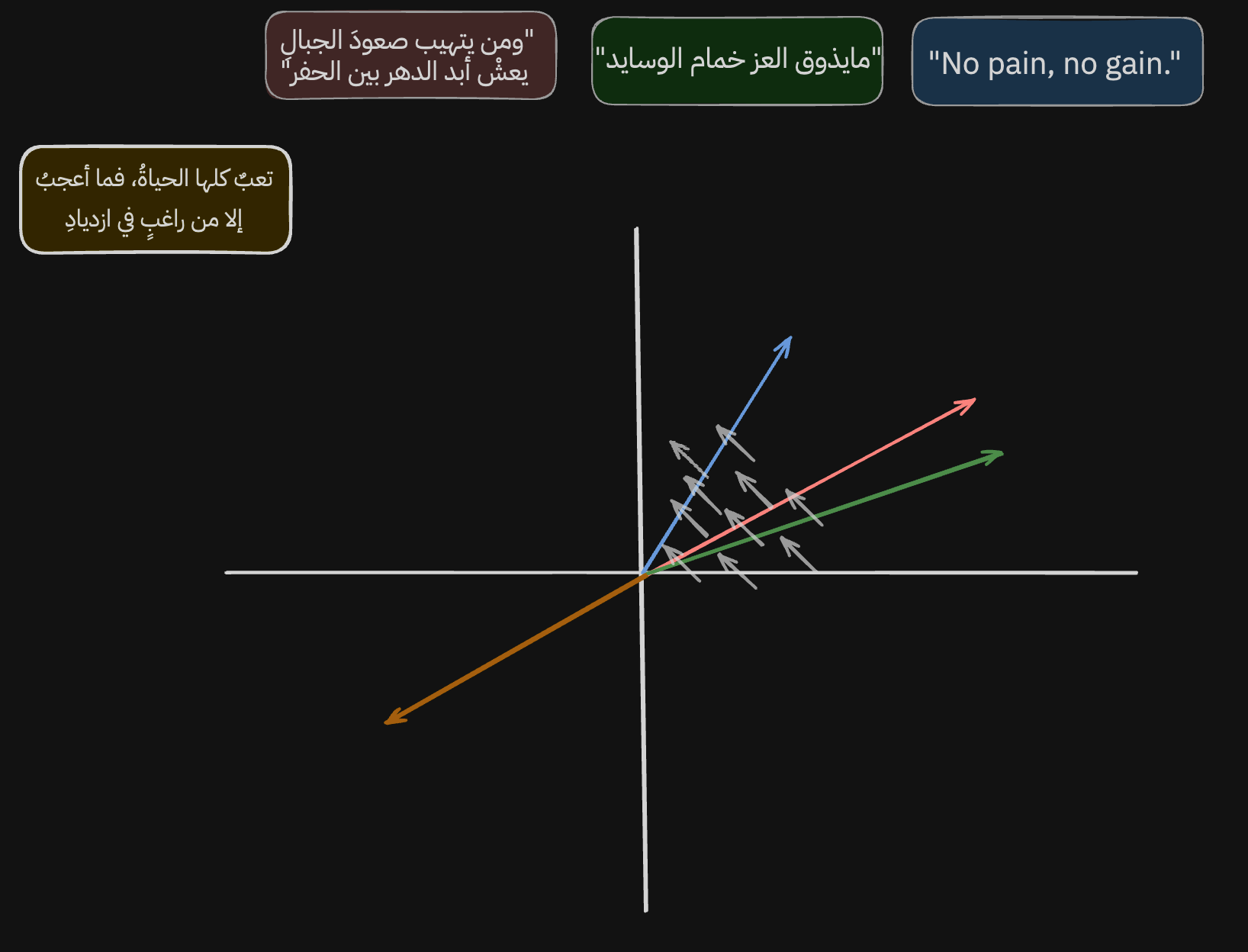
Not only that. In this image, and in this direction, the model learned to represent the shift from colloquial Arabic to formal Arabic to English.

This is a small part of the power of vectors and embeddings. Once we understand this idea, we can use it in many kinds of systems. Today, we will use it to strengthen traditional keyword search with semantic search, producing a search experience that uses both exact words and vectors that represent context.

Another image to make the idea clearer:

The Search Engine

Before we start building, let's set a few basic rules and requirements.

• The search engine has to mix keyword search with semantic search. Why? Because semantic search depends on meaning, not the exact word itself. That is not always the best approach when we are searching for something precise. Let's take a few example questions and results. Assume we have stored responses and the search engine's job is to return the correct response.

Question: "Article 13 of the Saudi Companies Law."

Keyword search: "Article 13 of the Companies Law states that..."

Semantic search: "The general law includes provisions related to limited liability companies..."

Here, keyword search gives us the better answer because it focuses on exact matching. Semantic search fails even though it returns something close in meaning.

Question: "Pain near the heart but not the heart."

Keyword search: "A heart attack causes chest pain..."

Semantic search: "Pain on the left side may be caused by stomach or muscle issues, not the heart."

Here, keyword search fails because it depends on matching, not understanding context. Semantic search gives the better answer. It also handles spelling mistakes much better than keyword search.

Each search method has strengths and weaknesses. The question we want to answer is: what happens if we combine them?

• The search engine must be good in Arabic, obviously.

• We need to simulate reality. In production, especially because we are representing podcast episodes, the number of items can be huge. PodcastIndex has more than 100 million episodes. So the model needs to be cheap, small, and fast.

Let's begin.

1. Download Podcasts and Episodes Locally

In this step, I use PodcastIndex. It is a decentralized, open podcast database with a simple API. We will pull its data into a local database.

I will only share small code examples here so the article does not turn into a mess. The full code is open source, and you can check it in this repo.

for query in queries:

	search_results, search_raw = search_podcasts(index, query, clean=True)

	...

The script in scripts/load_from_index.py pulls data in two ways. The first is through queries: specific podcasts I want to force into the dataset. We will see why in a bit.

The second way is pulling trending podcasts under specific categories. For some reason, PodcastIndex sometimes marks podcasts nobody knows as trending, so I keep a separate query list for the podcasts I definitely want included.

# These are from https://api.podcastindex.org/api/1.0/categories/list?pretty (Auth needed)

top_podcast_categories = {

    "News": 55,

    "True Crime": 103,

    "Comedy": 16,

    "Society": 77,

    "Culture": 78,

    ...

}

for cat in top_podcast_categories:

	trending_results, trending_raw = get_trending_podcasts(

		index,

		language=[lang],

		max_results=50,

		categories=[top_podcast_categories[cat]],

		since=timestamp_2024_01_01,

	)

	...

After we pull the data and store it in a local database, we move to the interesting part: embedding and encoding it.

Before we start, we need to talk about a different kind of database: vector databases. In short, these databases are built from the ground up for working with vectors. To make the difference clearer, look at the next image.

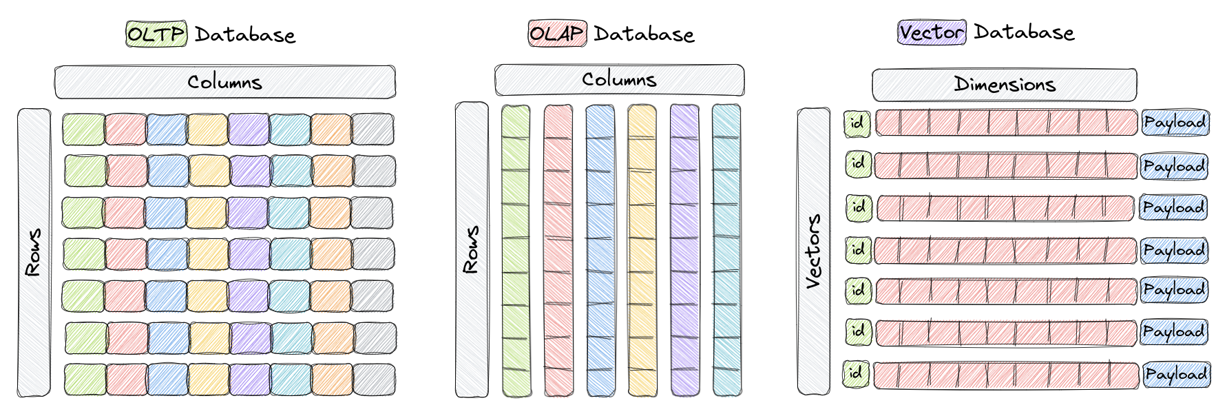
Here we see the difference between OLTP, the normal and familiar kind of database like Postgres, where data is structured as rows, and OLAP, where data is stored as columns. OLTP is good at fast inserts and reads, but it is less efficient for analytics and mathematical operations. OLAP is highly efficient for analytics and computation. Imagine we have 1,000 columns and need to run a mathematical operation. In OLTP, we often end up reading many columns to get what we need, which is slower and takes more space. In OLAP, because data is stored by column, we can pull only the columns needed for the operation. That is much more efficient. Of course, it has tradeoffs too, like slower writes and reads for some workloads.

Then comes the new type: a database structured around vectors. It is not organized around rows and columns in the same way. To explain it simply, I will use the database we are using here: Qdrant. There are many vector databases, and each has its advantages. I like Qdrant because the developer experience is good, the documentation is excellent, and the performance is strong.

How does Qdrant work under the hood, in a very simplified way?

We have two options: store the data on disk or keep it in memory. By default, vectors live directly in RAM, and the payload metadata lives there too. This is very fast, but not always practical.

When we choose on-disk storage, vectors are stored using memory-mapped files, or memmap. Let's unpack what is happening.

First, data in RAM is ideal for performance because access is fast and manipulation is efficient. What we want is something close to RAM performance while still storing the data on disk.

We start by storing the vectors sequentially with a fixed size in a file like this:

[vector_1][vector_2][vector_3]...[vector_n]

These vectors are stored in their simple raw form. Then we use the mmap system call, which maps this file into virtual memory space. Virtual memory is an abstraction that connects physical RAM to a virtual space that can be larger than the actual physical memory. When something needs to be in RAM, the system can pull in only the part we need.

In the vector example, when we call mmap, the system maps the file to a contiguous region in virtual memory. The file is split into pages, and each page corresponds to a section in virtual memory. Usually, each page is 4KB. When we need something from the file, instead of loading the whole file into RAM, we only load the page we need. Because the vectors are stored sequentially and have a fixed size, the calculation is simple. For example: offset = index * vector_size * sizeof(float32). This lets us load only the relevant piece into RAM and get performance close to keeping everything in memory.

That covers vectors. What about payloads or metadata? They are useful when we want to store descriptions for each vector, mostly for filtering, or when we want to store IDs that point to actual rows in a normal database.

These descriptions are stored in a key-value store. In Qdrant's case, they use RocksDB for this.

Back to the code.

Let's look at what happens in scripts/load_to_vdb.py.

First, we need to run a Qdrant container. I put it in docker-compose.

  qdrant:

    image: qdrant/qdrant:latest

    restart: always

    container_name: better_search_qdrant

    ports:

      - "6333:6333"

      - "6334:6334"

    expose:

      - "6333"

      - "6334"

      - "6335"

    configs:

      - source: qdrant_config

        target: /qdrant/config/production.yaml

    volumes:

      - qdrant-data:/qdrant/storage

    networks:

      - better_network

Then we connect the Qdrant client.

For the URL, if you are running the code from inside the container, use "http://host.docker.internal:6333". If you are running it from outside the container, use "http://localhost:6333".

qdrant_client = QdrantClient(url=settings.QDRANT_BASE_URL)

Then we pull a group of podcasts and all their episodes from our database and clean them. I chose a smaller group of Arabic podcasts, then prepared each document, which will later be saved as a vector, so it includes the podcast name, its producer, the episode title, and the episode description. Why? Because I want the vector to carry that context and improve search accuracy.

podcast_ids = list(range(50, 86)) + list(range(97, 128))

with get_db_context() as session:

	logger.info(f"Loading episodes from db for {len(podcast_ids)} podcast")

	episodes = get_podcast_with_episodes(podcast_ids, session)

	logger.info(f"Loaded {len(episodes)} episode successfully")

logger.info("Preparing documents for embedding")

docs = [

	f"{normalize_arabic(episode.podcast_name)}\n{normalize_arabic(episode.podcast_author)}\n{normalize_arabic(episode.title)}\n{clean_description(episode.description)}"

	for episode in episodes

]

Now we have two paths, because we said our search should mix keyword search and semantic search. There are two terms we should define.

The first is dense vectors. These are the vectors we have been talking about this whole time, shaped like [12, -3.3, 0.24, .....]. They are full of numbers and are excellent at preserving context.

The second is sparse vectors. These help preserve keywords. They are huge vectors, as large as the vocabulary in your data. If your data has 43,000 terms, the vector has 43,000 dimensions. They are called sparse because most values are zero. If we give it the sentence "مايذوق العز خمام الوسايد", only the indices corresponding to those words get a value. Example:

[0, 0, 2.5, 0, 0, 0, 0, 1.8, 0, 0, 0, 0, 0, 3.1, 0, 0, ....., 0, 0, 0, 0, 0]

Of course, for efficiency, the data is not stored like that. Only the positions and their values are stored, like {2:2.5, 7:1.8, 14:3.1}. The values are determined by the algorithm. In our example, we use BM25: an old, fast, simple, and excellent algorithm. It is similar to TF-IDF if you know it, but improves on it.

For dense vectors, we have two options: use a small, fast local model, or use an OpenAI embedding model, which is larger and higher quality but not local.

    if embedding_type == "local":

        handle_local_embeddings(

            qdrant_client=qdrant_client,

            collection_name=collection_name,

            documents=docs,

            episodes=episodes,

        )

    else:

        handle_openai_embeddings(

            qdrant_client=qdrant_client,

            collection_name=collection_name,

            documents=docs,

            episodes=episodes,

        )

Based on your choice, we go down one of these paths. Both serve the same goal. Let's look at the local path because Qdrant's abstraction makes the code cleaner and simpler.

def handle_local_embeddings(

    qdrant_client: QdrantClient,

    collection_name: str,

    documents: list[str],

    episodes: list[EpisodeInfo],

):

    qdrant_client.set_model(settings.LOCAL_EMBEDDING_MODEL)

    qdrant_client.set_sparse_model(settings.SPARSE_EMBEDDING_MODEL)

    if not qdrant_client.collection_exists(collection_name):

        qdrant_client.create_collection(

            collection_name=collection_name,

            vectors_config=qdrant_client.get_fastembed_vector_params(),

	    sparse_vectors_config=qdrant_client.get_fastembed_sparse_vector_params(),

        )

    qdrant_client.add(

        collection_name=collection_name,

        documents=documents,

        metadata=[

        episode.model_dump(exclude={"description"})

        for episode in episodes],

        parallel=2,

        ids=tqdm(range(len(documents))),

    )

For the dense vector, we used paraphrase-multilingual-MiniLM-L12-v2. Pay attention to whether the model you use supports Arabic. This is a small model with 384 dimensions, which is not huge. The OpenAI model we use has 1536 dimensions. Generally, more dimensions can improve representation, but they also increase storage. OpenAI has models with 3072 dimensions too, and there are open-source models in that range as well.

As you can see, embedding the data and adding it to the vector database is very simple. The OpenAI code is simple too, but we have to do a few steps ourselves because Qdrant does not provide automatic OpenAI support inside this abstraction.

Now, if you go to http://localhost:6333/dashboard#/collections/, you should see your data.

All that remains is the method that lets a user send a query and run the search operation, with Qdrant doing most of the heavy lifting. Let's create HybridSearcher.

A simple definition of what we need:

class HybridSearch:

    def init(

        self,

        collection_name: str,

        url: str = settings.QDRANT_BASE_URL,

        mode: Annotated[str, "either 'openai' or 'local'"] = "local",

    ):

        self.collection_name = collection_name

        self.client = QdrantClient(url=url)

        self.mode = mode

        if mode == "local":

            self.DENSE_MODEL = TextEmbedding(settings.LOCAL_EMBEDDING_MODEL)

        else:

            self.DENSE_MODEL = OpenAI(api_key=settings.OPENAI_API_KEY)

        self.SPARSE_MODEL = Bm25(settings.SPARSE_EMBEDDING_MODEL)

Now for the important part: the search function. First, it calls _get_query_embeddings, a small helper that keeps the code clean when switching between a local model and OpenAI.

    def search(self, query: str):

        query_dense_vector, query_sparse_vector = self._get_query_embeddings(query)

        prefetch = self._get_prefetch(

            length=len(query.split()),

            query=query,

            query_dense_vector=query_dense_vector,

            query_sparse_vector=query_sparse_vector,

        )

        result = self.client.query_points(

            collection_name=self.collection_name,

            prefetch=prefetch,

            query=models.FusionQuery(fusion=models.Fusion.RRF),

            limit=10,

            with_payload=True,

        )

        response = [

            HybridSearchResult(

                podcast_id=r.payload["podcast_id"],

                episode_id=r.payload["episode_id"],

                episode_title=r.payload["document"].split("\n")[2],

                podcast_title=r.payload["podcast_name"],

                podcast_author=r.payload["podcast_author"],

                podcast_categoires=r.payload["podcast_categories"],

                sim_score=r.score,

            )

            for r in result.points

        ]

        return response

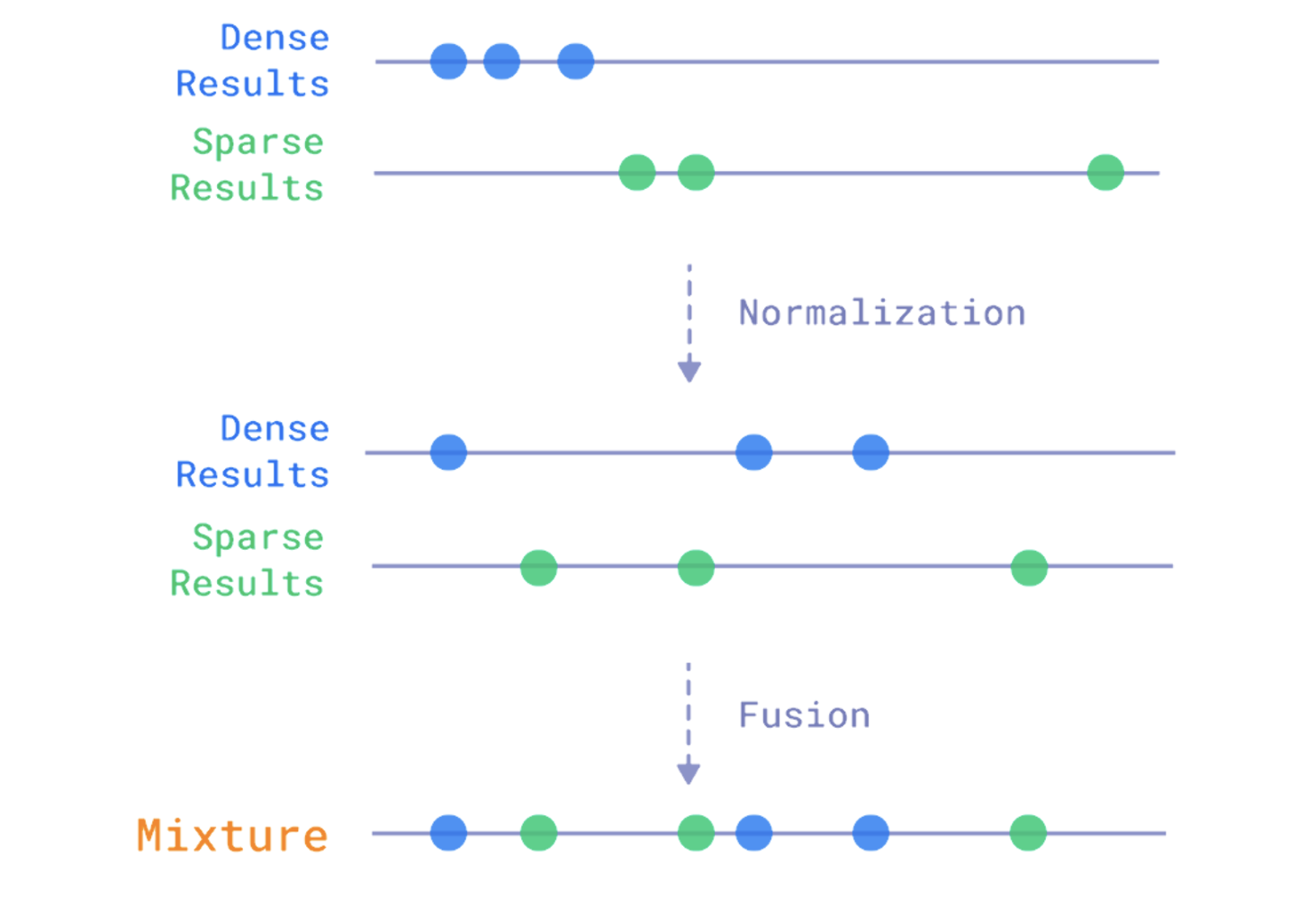
Then it calls another helper. Prefetch is how we tell Qdrant what we want to request from the database and how we want the data to come back. Qdrant then handles the search according to the plan we gave it. Here we choose when to use dense vectors, when to use sparse vectors, how to mix them, how many results we want back, and a few other details. Sometimes we query the same vector twice. For example, when the query is shorter than three words, we use sparse search twice and add a filter in the second pass. The hybrid part happens when we search both ways, semantic and keyword, then merge them at the end using fusion in the final query_points call. The next image makes this clearer.

 def getprefetch(

        self,

        length: int,

        query: str,

        query_dense_vector: list[float],

        query_sparse_vector: list[float],

    ):

        if length <= 3:

            prefetch = [

                models.Prefetch(

                    query=models.SparseVector(**query_sparse_vector.as_object()),

                    using="bm25",

                    limit=40,

                    params=models.SearchParams(hnsw_ef=256, exact=True),

                ),

                models.Prefetch(

                    query=models.SparseVector(**query_sparse_vector.as_object()),

                    using="bm25",

                    limit=40,

                    params=models.SearchParams(hnsw_ef=256, exact=True),

                    filter=models.Filter(

                        should=models.FieldCondition(

                            key="documents", match=models.MatchAny(any=query.split())

                        )

                    ),

                ),

            ]

        else:

            prefetch = [

                models.Prefetch(

                    query=query_dense_vector,

                    using=(

                        "openai"

                        if self.mode == "openai"

                        else "fast-paraphrase-multilingual-minilm-l12-v2"

                    ),

                    limit=15,

                    params=models.SearchParams(

                        hnsw_ef=256,

                        exact=True,

                    ),

                ),

                models.Prefetch(

                    query=models.SparseVector(**query_sparse_vector.as_object()),

                    using="bm25",

                    limit=40,

                    params=models.SearchParams(hnsw_ef=256, exact=True),

                ),

                models.Prefetch(

                    query=models.SparseVector(**query_sparse_vector.as_object()),

                    using="bm25",

                    limit=40,

                    params=models.SearchParams(hnsw_ef=256, exact=True),

                    filter=models.Filter(

                        should=models.FieldCondition(

	                            key="documents", match=models.MatchAny(any=query.split())

                        )

                    ),

                ),

            ]

        return prefetch

I have a simple condition here: if the search query has fewer than four words, we only use keyword search because it is usually more precise. Once the query gets longer, we start using the hybrid mix.

There are two common ways to combine the results of the two searches. The first is fusion, which is what we use here. The idea is simple: combine based on the results returned by each search. Vectors that come back with high similarity rise in the final result.

The second method, which we are not using here, is re-ranking. Usually, this uses a model whose main job is to reorder results based not only on the score, but also on a fresh pass over the vectors and a few other signals.

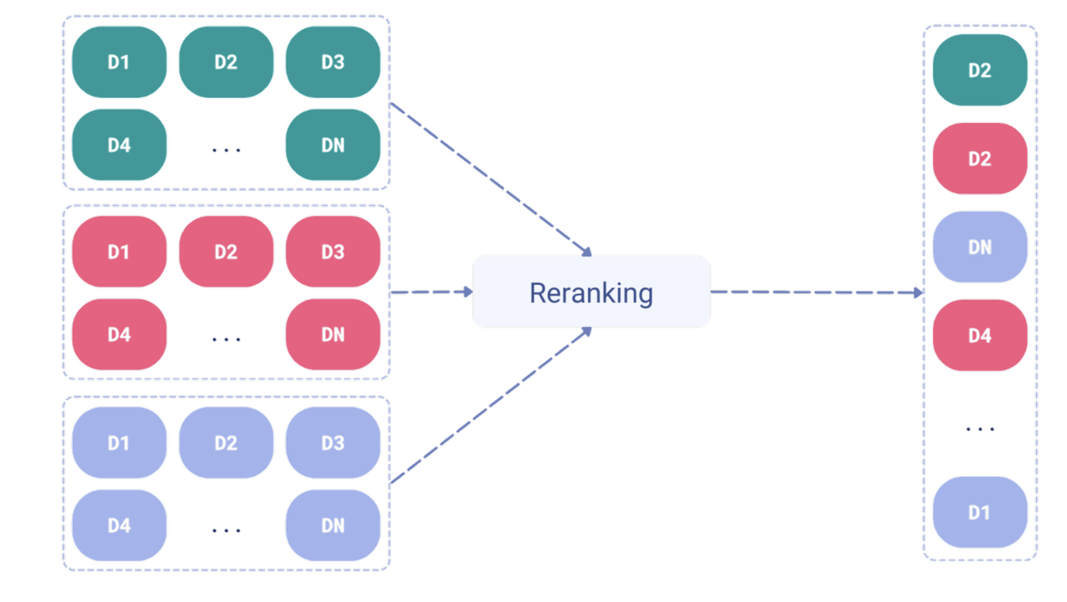
Both methods have pros and cons. The first is faster, but can lose some accuracy. The second is more accurate, but slower.

Yes, we skipped a few things in the code, but everything is in the repo if you want to check it. And honestly, once we reach this point, the engine is already implemented with surprising simplicity, thanks to Qdrant doing the heavy lifting. You can connect it to an API and a frontend and have a strong search engine. The API and frontend code I have is just enough to run a demo, so do not build your production system on that part.

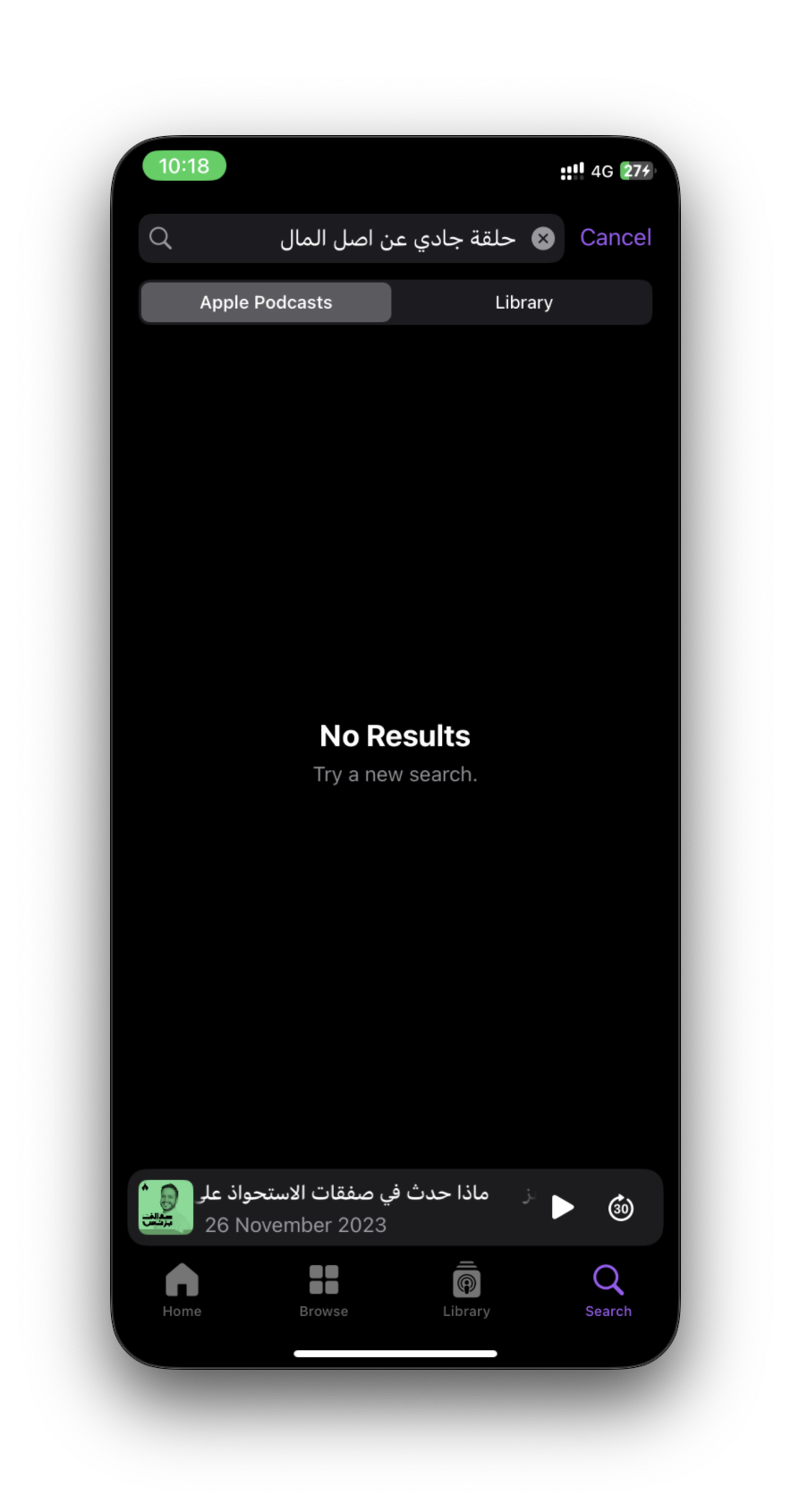
Let's search, for example, for "the Jadi episode about the origin of money."

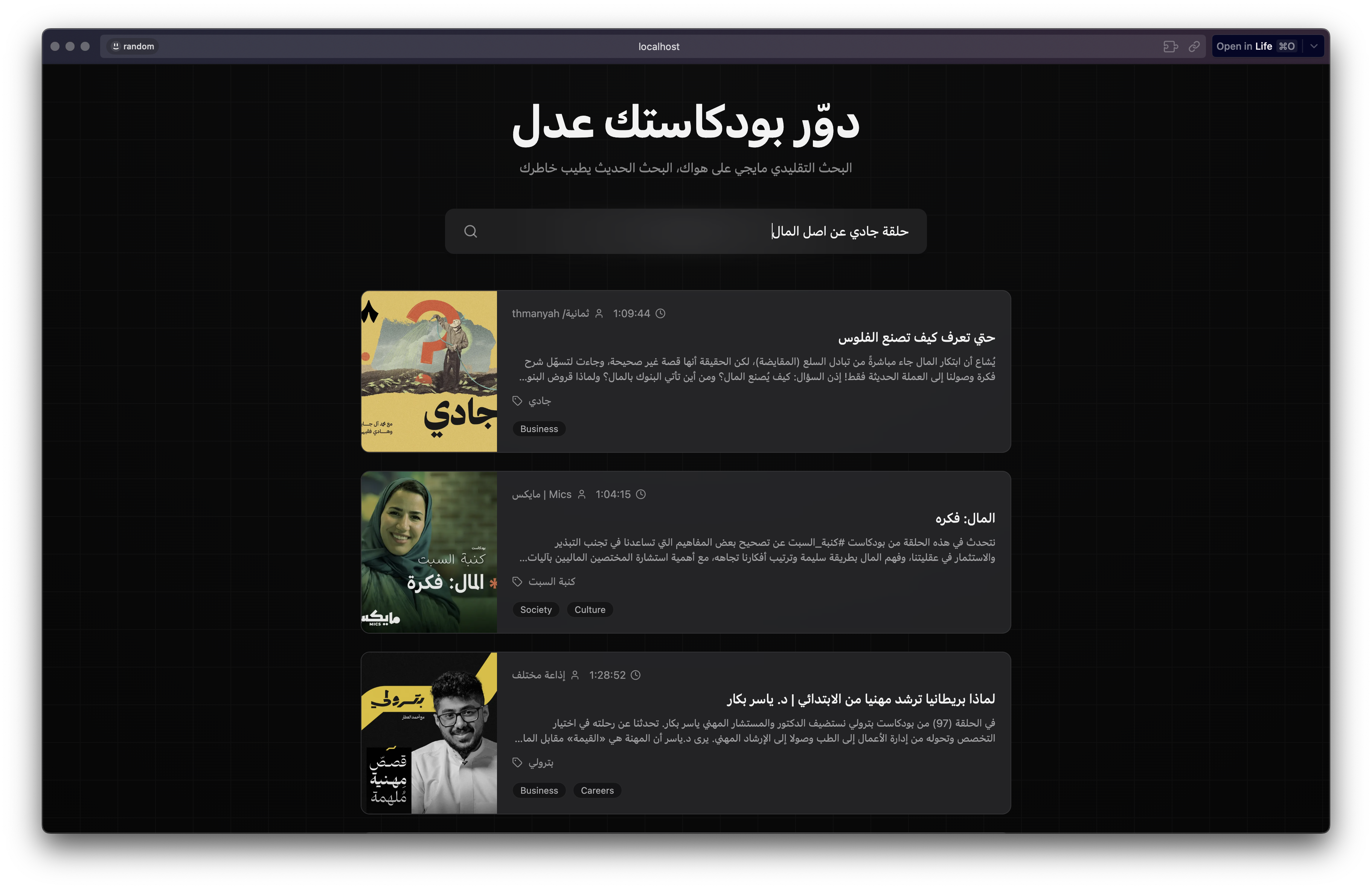
We find what we want even though the phrase "origin of money" is not in the episode description or title. If we run the same search in Radio Thmanyah or Apple Podcasts, we do not find the intended episode.

We could try more examples, but I think the idea is clear. This approach has advantages, and sometimes disadvantages, because it may rank more than one episode highly based on context. But most of the time, it gets you what you want better than traditional search. Of course, there are challenges when applying this at large scale. As we saw, PodcastIndex has more than 100 million episodes, and with a number that large, semantic search quality may start to drop.

There are interesting ideas worth exploring here. Right now, we only embed the episode description. What if we embedded the whole episode? What if we took the transcript and represented the entire thing, so when we search for something we saw in a short clip or reel, we can still find it even if our question is nowhere near the title or description? Of course, the scale for that is wild and not practical at all, but it is interesting to think about.

Interesting Points

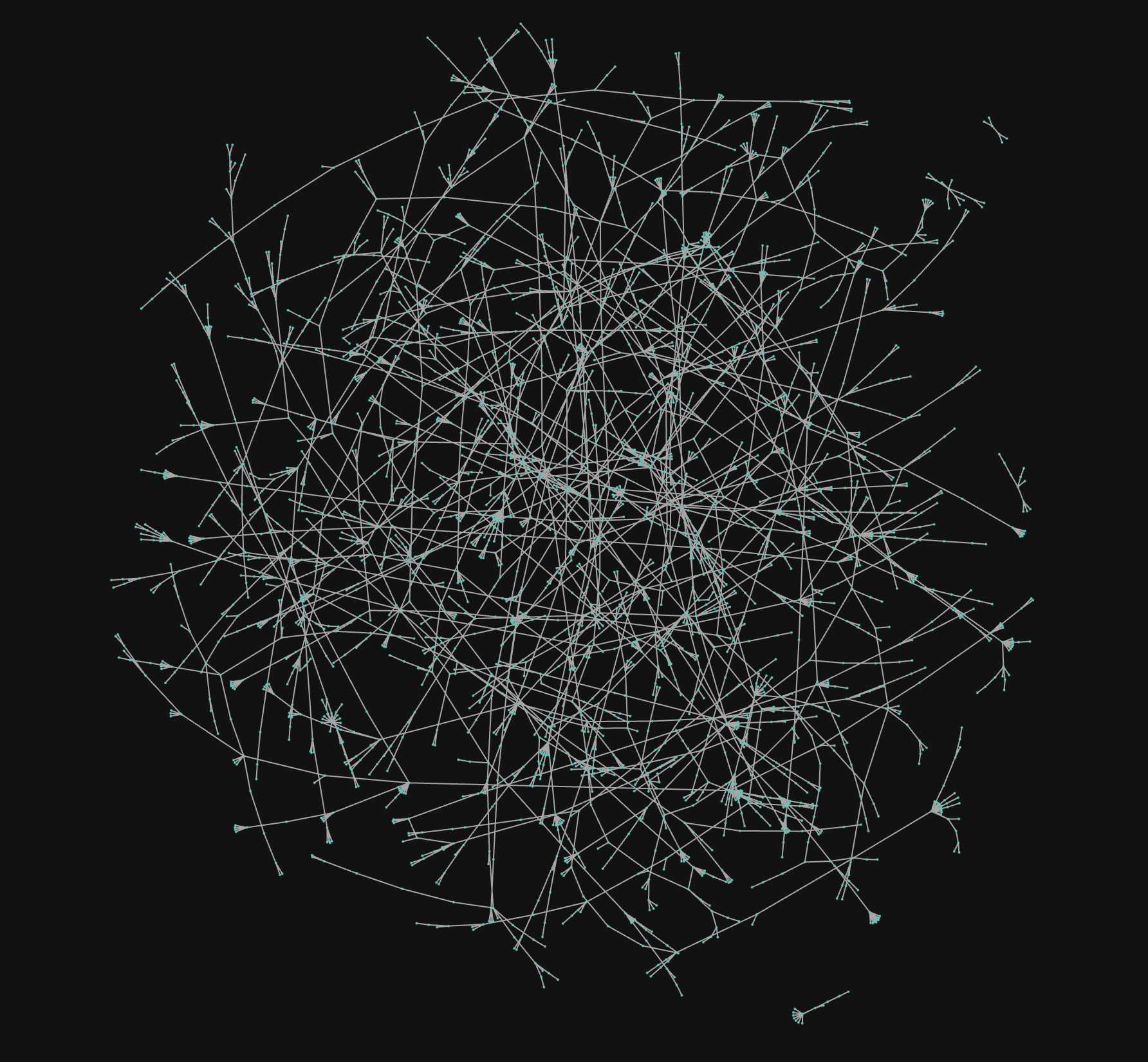
This image represents vectors for 3,000 episodes. When we zoom in, we discover interesting things using what we learned earlier about vectors and representation.

Let's pick one of these regions and see which episodes clustered together.

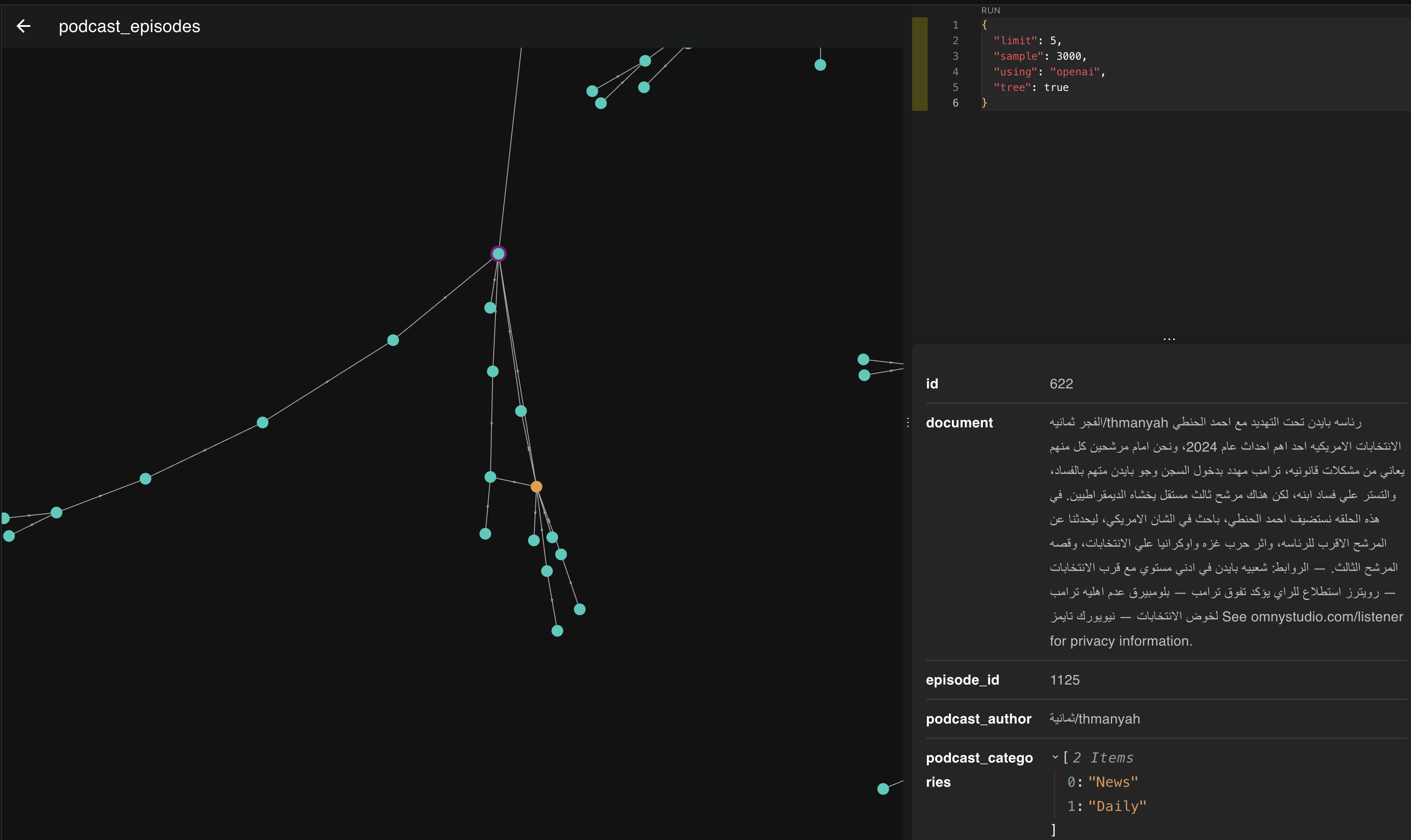
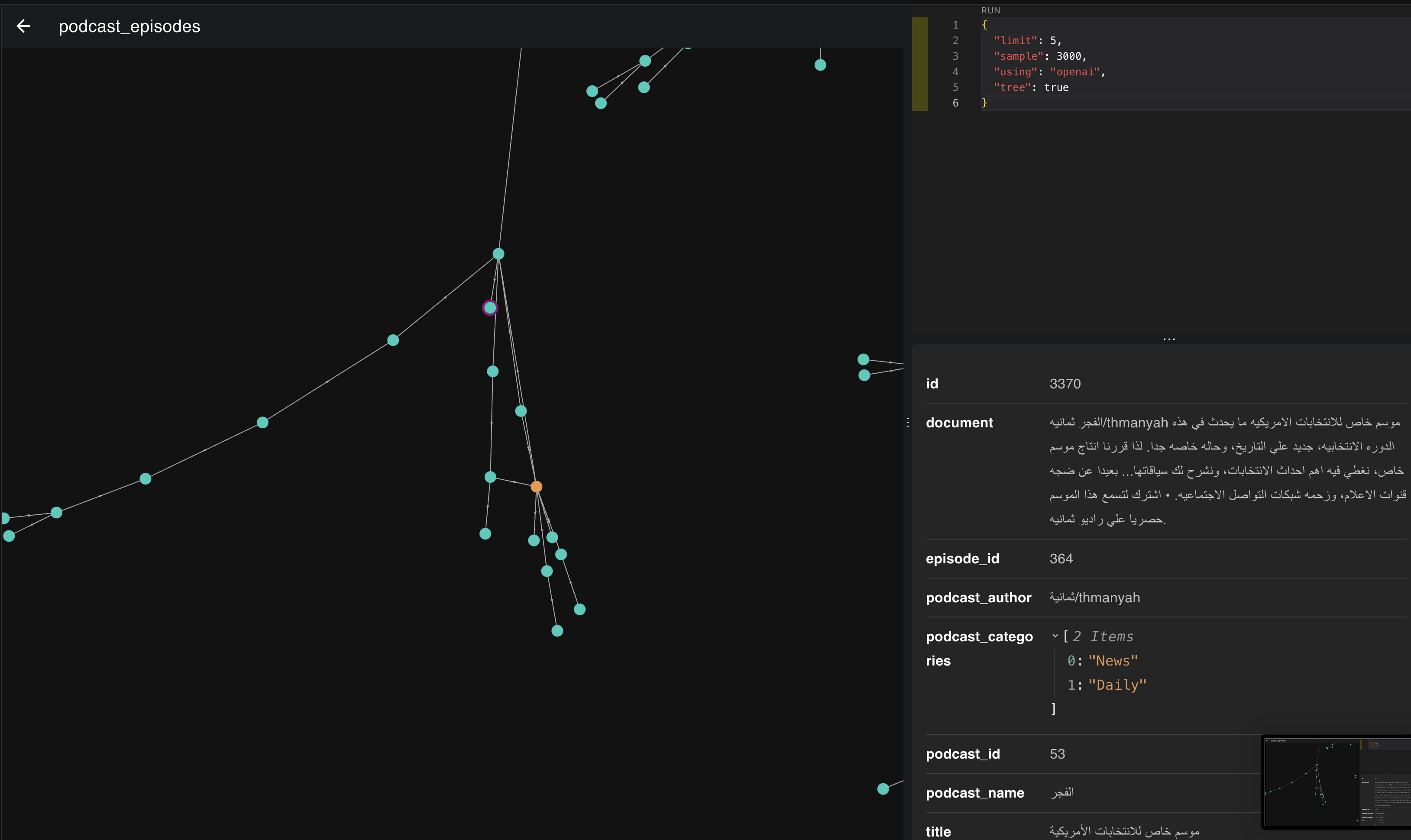
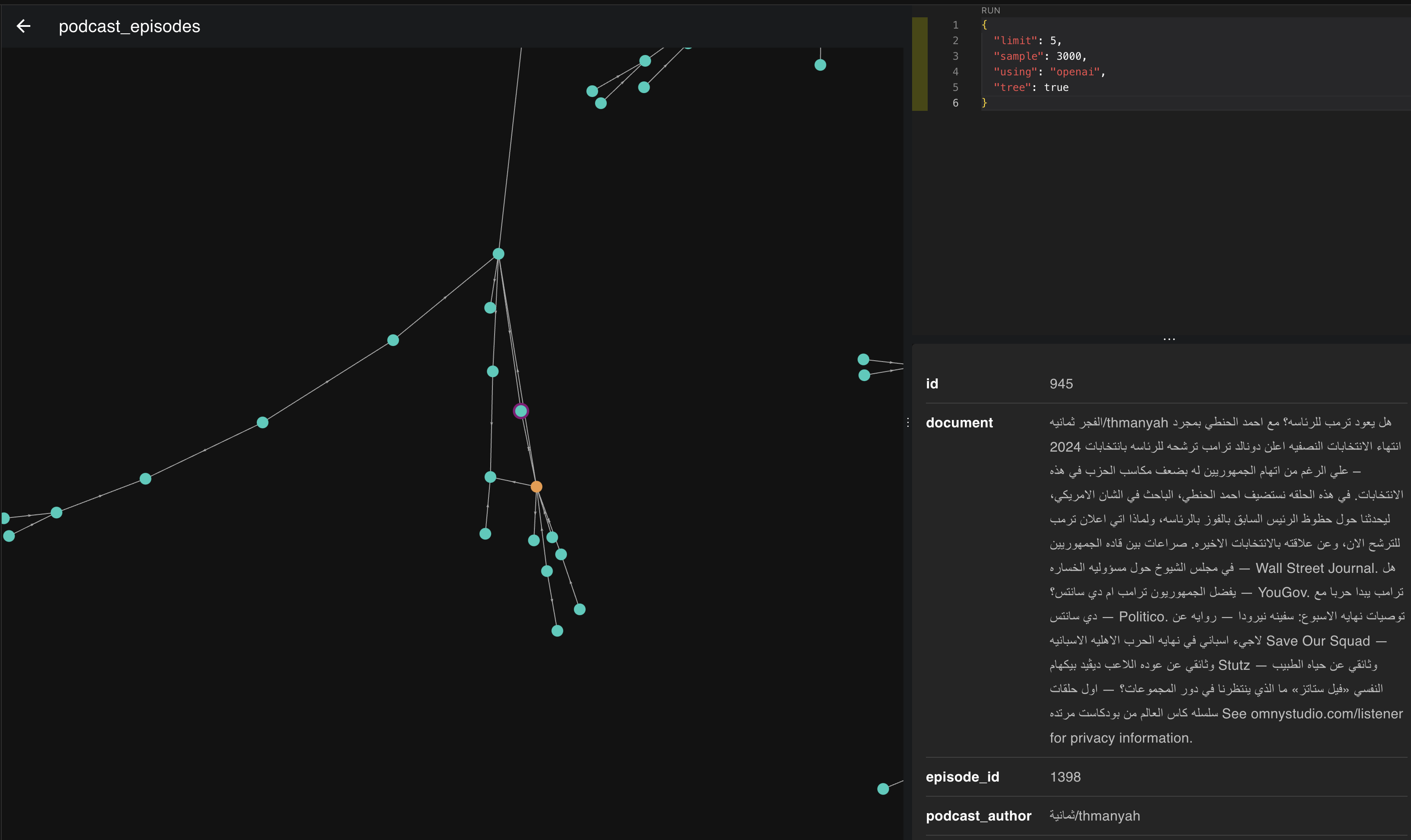
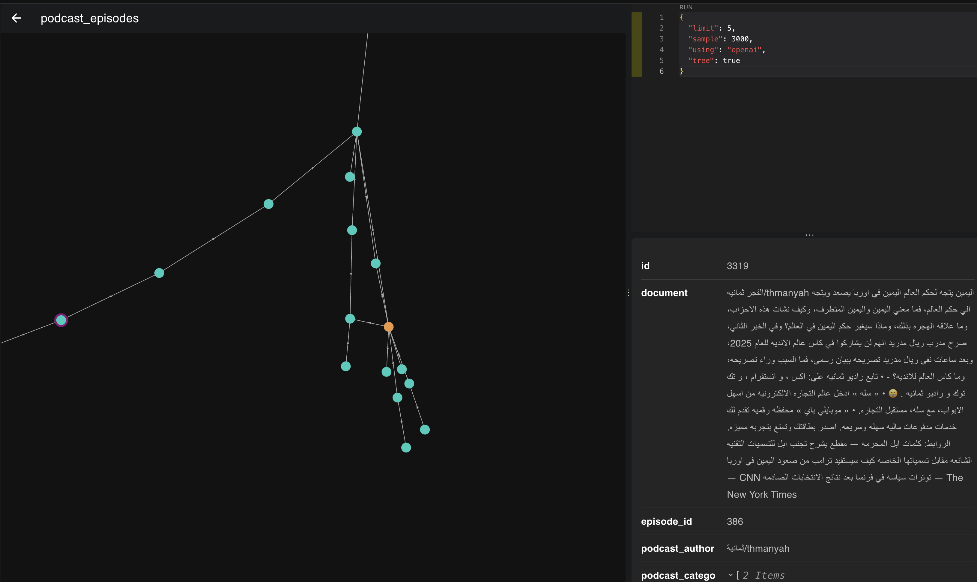
If we look at the images above, the episodes clustered in this place and direction are all about politics and heads of state. The more we move down to the right, the more the topic becomes America and its president. If we move slightly left, we start moving toward Europe and its presidents.

This is another excellent use of vectors and embeddings: they help you build strong recommendation systems. If you see users listening to certain episodes a lot, you can recommend nearby episodes and give them a much better experience.

The Takeaway

There is much more to say, and many more conclusions we could draw from this topic, but we will stop here. I hope the core idea is clear, and that the value of vectors and embeddings is clear too. This was only one angle on the topic.

More to come.